This is part 1 of a series of blog posts about MCMC techniques:

• Part II: Gibbs sampling
• Part III: Hamiltonian Monte Carlo
• Part IV: Replica Exchange

Markov chain Monte Carlo (MCMC) is a powerful class of methods to sample from probability distributions known only up to an (unknown) normalization constant. But before we dive into MCMC, let’s consider why you might want to do sampling in the first place.

The answer to that is: whenever you’re either interested in the samples themselves (for example, inferring unknown parameters in Bayesian inference) or you need them to approximate expected values of functions w.r.t. to a probability distribution (for example, calculating thermodynamic quantities from the distribution of microstates in statistical physics). Sometimes, only the mode of a probability distribution is of primary interest. In this case, it’s obtained by numerical optimization so full sampling is not necessary.

It turns out that sampling from any but the most basic probability distributions is a difficult task. Inverse transform sampling is an elementary method to sample from probability distributions, but requires the cumulative distribution function, which in turn requires knowledge of the, generally unknown, normalization constant. Now in principle, you could just obtain the normalization constant by numerical integration, but this quickly gets infeasible with an increasing number of dimensions. Rejection sampling does not require a normalized distribution, but efficiently implementing it requires a good deal of knowledge about the distribution of interest, and it suffers strongly from the curse of dimension, meaning that its efficiency decreases rapidly with an increasing number of variables. That’s when you need a smart way to obtain representative samples from your distribution which doesn’t require knowledge of the normalization constant.

MCMC algorithms are a class of methods which do exactly that. These methods date back to a seminal paper by Metropolis et al., who developed the first MCMC algorithm, correspondingly called Metropolis algorithm, to calculate the equation of state of a two-dimensional system of hard spheres. In reality, they were looking for a general method to calculate expected values occurring in statistical physics.

In this blog post, I introduce the basics of MCMC sampling; in subsequent posts I’ll cover several important, increasingly complex and powerful MCMC algorithms, which all address different difficulties one frequently faces when using the Metropolis-Hastings algorithm. Along the way, you will gain a solid understanding of these challenges and how to address them. Also, this serves as a reference for MCMC methods in the context of the monad-bayes series. Furthermore, I hope the provided notebooks will not only spark your interest in exploring the behavior of MCMC algorithms for various parameters/probability distributions, but also serve as a basis for implementing and understanding useful extensions of the basic versions of the algorithms I present.

Markov chains

Now that we know why we want to sample, let’s get to the heart of MCMC: Markov chains. What is a Markov chain? Without all the technical details, a Markov chain is a random sequence of states in some state space in which the probability of picking a certain state next depends only on the current state in the chain and not on the previous history: it is memory-less. Under certain conditions, a Markov chain has a unique stationary distribution of states to which it converges after a certain number of states. From that number on, states in the Markov chain are distributed according to the invariant distribution.

In order to sample from a distribution $\pi(x)$, a MCMC algorithm constructs and simulates a Markov chain whose stationary distribution is $\pi(x)$, meaning that, after an initial “burn-in” phase, the states of that Markov chain are distributed according to $\pi(x)$. We thus just have to store the states to obtain samples from $\pi(x)$.

For didactic purposes, let’s for now consider both a discrete state space and discrete “time”. The key quantity characterizing a Markov chain is the transition operator $T(x_{i+1}|x_i)$ which gives you the probability of being in state $x_{i+1}$ at time $i+1$ given that the chain is in state $x_i$ at time $i$.

Now just for fun (and for illustration), let’s quickly whip up a Markov chain which has a unique stationary distribution. We’ll start with some imports and settings for the plots:

%matplotlib notebook
%matplotlib inline
import numpy as np
import matplotlib.pyplot as plt
plt.rcParams['figure.figsize'] = [10, 6]
np.random.seed(42)

The Markov chain will hop around on a discrete state space which is made up from three weather states:

state_space = ("sunny", "cloudy", "rainy")

In a discrete state space, the transition operator is just a matrix. Columns and rows correspond, in our case, to sunny, cloudy, and rainy weather. We pick more or less sensible values for all transition probabilities:

transition_matrix = np.array(((0.6, 0.3, 0.1),
                              (0.3, 0.4, 0.3),
                              (0.2, 0.3, 0.5)))

The rows indicate the states the chain might currently be in and the columns the states the chains might transition to. If we take one “time” step of the Markov chain as one hour, then, if it’s sunny, there’s a 60% chance it stays sunny in the next hour, a 30% chance that in the next hour we will have cloudy weather, and only a 10% chance of rain immediately after it had been sunny before. This also means that each row has to sum up to one.

Let’s run our Markov chain for a while:

n_steps = 20000
states = [0]
for i in range(n_steps):
    states.append(np.random.choice((0, 1, 2), p=transition_matrix[states[-1]]))
states = np.array(states)

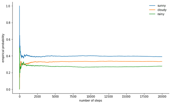
We can monitor the convergence of our Markov chain to its stationary distribution by calculating the empirical probability for each of the states as a function of chain length:

def despine(ax, spines=('top', 'left', 'right')):
    for spine in spines:
        ax.spines[spine].set_visible(False)

fig, ax = plt.subplots()
width = 1000
offsets = range(1, n_steps, 5)
for i, label in enumerate(state_space):
    ax.plot(offsets, [np.sum(states[:offset] == i) / offset
            for offset in offsets], label=label)
ax.set_xlabel("number of steps")
ax.set_ylabel("likelihood")
ax.legend(frameon=False)
despine(ax, ('top', 'right'))
plt.show()

The mother of all MCMC algorithms: Metropolis-Hastings

So that’s lots of fun, but back to sampling an arbitrary probability distribution $\pi$. It could either be discrete, in which case we would keep talking about a transition matrix $T$, or be continuous, in which case $T$ would be a transition kernel. From now on, we’re considering continuous distributions, but all concepts presented here transfer to the discrete case.

If we could design the transition kernel in such a way that the next state is already drawn from $\pi$, we would be done, as our Markov chain would… well… immediately sample from $\pi$. Unfortunately, to do this, we need to be able to sample from $\pi$, which we can’t. Otherwise you wouldn’t be reading this, right?

A way around this is to split the transition kernel $T(x_{i+1}|x_i)$ into two parts: a proposal step and an acceptance/rejection step. The proposal step features a proposal distribution $q(x_{i+1}|x_i)$, from which we can sample possible next states of the chain. In addition to being able to sample from it, we can choose this distribution arbitrarily. But, one should strive to design it such that samples from it are both as little correlated with the current state as possible and have a good chance of being accepted in the acceptance step. Said acceptance/rejection step is the second part of the transition kernel and corrects for the error introduced by proposal states drawn from $q \neq \pi$. It involves calculating an acceptance probability $p_\mathrm{acc}(x_{i+1}|x_i)$ and accepting the proposal $x_{i+1}$ with that probability as the next state in the chain. Drawing the next state $x_{i+1}$ from $T(x_{i+1}|x_i)$ is then done as follows: first, a proposal state $x_{i+1}$ is drawn from $q(x_{i+1}|x_i)$. It is then accepted as the next state with probability $p_\mathrm{acc}(x_{i+1}|x_i)$ or rejected with probability $1-p_\mathrm{acc}(x_{i+1}|x_i)$, in which case the current state is copied as the next state.

We thus have

A sufficient condition for a Markov chain to have $\pi$ as its stationary distribution is the transition kernel obeying detailed balance or, in the physics literature, microscopic reversibility:

This means that the probability of being in a state $x_i$ and transitioning to $x_{i+1}$ must be equal to the probability of the reverse process, namely, being in state $x\_{i+1}$ and transitioning to $x_i$. Transition kernels of most MCMC algorithms satisfy this condition.

For the two-part transition kernel to obey detailed balance, we need to choose $p_\mathrm{acc}$ correctly, meaning that is has to correct for any asymmetries in probability flow from / to $x_{i+1}$ or $x_i$. Metropolis-Hastings uses the Metropolis acceptance criterion:

Now here’s where the magic happens: we know $\pi$ only up to a constant, but it doesn’t matter, because that unknown constant cancels out in the expression for $p_\mathrm{acc}$! It is this property of $p_\mathrm{acc}$ which makes algorithms based on Metropolis-Hastings work for unnormalized distributions. Often, symmetric proposal distributions with $q(x_i|x_{i+1})=q(x_{i+1}|x_i)$ are used, in which case the Metropolis-Hastings algorithm reduces to the original, but less general Metropolis algorithm developed in 1953 and for which

We can then write the complete Metropolis-Hastings transition kernel as

Implementing the Metropolis-Hastings algorithm in Python

All right, now that we know how Metropolis-Hastings works, let’s go ahead and implement it. First, we set the log-probability of the distribution we want to sample from—without normalization constants, as we pretend we don’t know them. Let’s work for now with a standard normal distribution:

def log_prob(x):
     return -0.5 * np.sum(x ** 2)

Next, we choose a symmetric proposal distribution. Generally, including information you have about the distribution you want to sample from in the proposal distribution will lead to better performance of the Metropolis-Hastings algorithm. A naive approach is to just take the current state $x$ and pick a proposal from $\mathcal{U}(x-\frac{\Delta}{2}, x+\frac{\Delta}{2})$, that is, we set some step size $\Delta$ and move left or right a maximum of $\frac{\Delta}{2}$ from our current state:

def proposal(x, stepsize):
    return np.random.uniform(low=x - 0.5 * stepsize,
                             high=x + 0.5 * stepsize,
                             size=x.shape)

Finally, we calculate our acceptance probability:

def p_acc_MH(x_new, x_old, log_prob):
    return min(1, np.exp(log_prob(x_new) - log_prob(x_old)))

Now, we piece all this together into our really brief implementation of a Metropolis-Hastings sampling step:

def sample_MH(x_old, log_prob, stepsize):
    x_new = proposal(x_old, stepsize)
    # here we determine whether we accept the new state or not:
    # we draw a random number uniformly from [0,1] and compare
    # it with the acceptance probability
    accept = np.random.random() < p_acc_MH(x_new, x_old, log_prob)
    if accept:
        return accept, x_new
    else:
        return accept, x_old

Apart from the next state in the Markov chain, x_new or x_old, we also return whether the MCMC move was accepted or not. This will allow us to keep track of the acceptance rate. Let’s complete our implementation by writing a function that iteratively calls sample_MH and thus builds up the Markov chain:

def build_MH_chain(init, stepsize, n_total, log_prob):

    n_accepted = 0
    chain = [init]

    for _ in range(n_total):
        accept, state = sample_MH(chain[-1], log_prob, stepsize)
        chain.append(state)
        n_accepted += accept

    acceptance_rate = n_accepted / float(n_total)

    return chain, acceptance_rate

Testing our Metropolis-Hastings implementation and exploring its behavior

Now you’re probably excited to see this in action. Here we go, taking some informed guesses at the stepsize and n_total arguments:

chain, acceptance_rate = build_MH_chain(np.array([2.0]), 3.0, 10000, log_prob)
chain = [state for state, in chain]
print("Acceptance rate: {:.3f}".format(acceptance_rate))
last_states = ", ".join("{:.5f}".format(state)
                        for state in chain[-10:])
print("Last ten states of chain: " + last_states)

Acceptance rate: 0.722
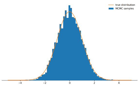
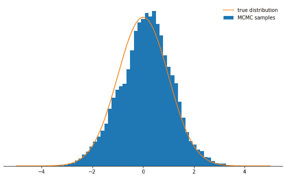
Last ten states of chain: -0.84962, -0.84962, -0.84962, -0.08692, 0.92728, -0.46215, 0.08655, -0.33841, -0.33841, -0.33841

All right. So did this work? We achieved an acceptance rate of around 71% and we have a chain of states. We should throw away the first few states during which the chain won’t yet have converged to its stationary distribution. Let’s check whether the states we drew are actually normally distributed:

def plot_samples(chain, log_prob, ax, orientation='vertical', normalize=True,
                 xlims=(-5, 5), legend=True):
    from scipy.integrate import quad

    ax.hist(chain, bins=50, density=True, label="MCMC samples",
           orientation=orientation)
    # we numerically calculate the normalization constant of our PDF
    if normalize:
        Z, _ = quad(lambda x: np.exp(log_prob(x)), -np.inf, np.inf)
    else:
        Z = 1.0
    xses = np.linspace(xlims[0], xlims[1], 1000)
    yses = [np.exp(log_prob(x)) / Z for x in xses]
    if orientation == 'horizontal':
        (yses, xses) = (xses, yses)
    ax.plot(xses, yses, label="true distribution")
    if legend:
        ax.legend(frameon=False)

fig, ax = plt.subplots()
plot_samples(chain[500:], log_prob, ax)
despine(ax)
ax.set_yticks(())
plt.show()

Looks great!

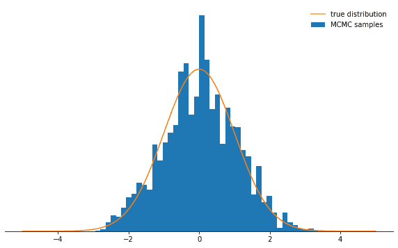
Now, what’s up with the parameters stepsize and n_total? We’ll discuss the step size first: it determines how far away a proposal state can be from the current state of the chain. It is thus a parameter of the proposal distribution $q$ and controls how big the random steps are which the Markov chain takes. If the step size is too large, the proposal state will often be in the tails of the distribution, where probability is low. The Metropolis-Hastings sampler rejects most of these moves, meaning that the acceptance rate decreases and convergence is much slower. See for yourself:

def sample_and_display(init_state, stepsize, n_total, n_burnin, log_prob):
    chain, acceptance_rate = build_MH_chain(init_state, stepsize, n_total, log_prob)
    print("Acceptance rate: {:.3f}".format(acceptance_rate))
    fig, ax = plt.subplots()
    plot_samples([state for state, in chain[n_burnin:]], log_prob, ax)
    despine(ax)
    ax.set_yticks(())
    plt.show()

sample_and_display(np.array([2.0]), 30, 10000, 500, log_prob)

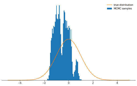
Acceptance rate: 0.116

Not as cool, right? Now you could think the best thing to do is do choose a tiny step size. Turns out that this is not too smart either because then the Markov chain will explore the probability distribution only very slowly and thus again won’t converge as rapidly as with a well-adjusted step size:

sample_and_display(np.array([2.0]), 0.1, 10000, 500, log_prob)

Acceptance rate: 0.992

No matter how you choose the step size parameter, the Markov chain will eventually converge to its stationary distribution. But it may take a looooong time. The time we simulate the Markov chain for is set by the n_total parameter—it simply determines how many states of the Markov chain (and thus samples) we’ll end up with. If the chain converges slowly, we need to increase n_total in order to give the Markov chain enough time to forget its initial state. So let’s keep the tiny step size and increase the number of samples by increasing n_total:

sample_and_display(np.array([2.0]), 0.1, 500000, 25000, log_prob)

Acceptance rate: 0.990

Sloooowly getting there…

Conclusions

With these considerations, I conclude the first blog post of this series. I hope you now understand the intuition behind the Metropolis-Hastings algorithm, its parameters, and why it is an extremely useful tool to sample from non-standard probability distributions you might encounter out there in the wild.

I highly encourage you to play around with the code provided in this notebook—this way, you can learn how the algorithm behaves in various circumstances and deepen your understanding of it. Go ahead and try out a non-symmetric proposal distribution! What happens if you don’t adjust the acceptance criterion accordingly? What happens if you try to sample from a bimodal distribution? Can you think of a way to automatically tune the stepsize? What are pitfalls here? Try it out and discover for yourself!

In my next post, I will discuss the Gibbs sampler—a special case of the Metropolis-Hastings algorithm that allows you to approximately sample from a multivariate distribution by sampling from the conditional distributions.

Thanks for reading—go forward and sample!