This is the third post of a series of blog posts about Markov Chain Monte Carlo (MCMC) techniques:
So far, we discussed two MCMC algorithms: the Metropolis-Hastings algorithm and the Gibbs sampler. Both algorithms can produce highly correlated samples—Metropolis-Hastings has a pronounced random walk behaviour, while the Gibbs sampler can easily get trapped when variables are highly correlated. In this blog post, we will take advantage of an additional piece of information about a distribution—its shape—and learn about Hamiltonian Monte Carlo, an algorithm whose roots are in quantum physics.
As always, you can download the corresponding IPython notebook and play around with the code to your heart’s desire!
Physical intuition
As mentioned above, when doing Metropolis-Hastings sampling with a naive proposal distribution, we are essentially performing a random walk without taking into account any additional information we may have about the distribution we want to sample from.
We can do better!
If the density function we want to sample from is differentiable, we have access to its local shape through its derivative.
This derivative tells us, at each point x, how the value of the density p(x) increases or decreases depending on how we change the x.
That means we should be able to use the derivative of p(x) to propose states with high probabilities—which is exactly the key idea of Hamiltonian Monte Carlo (HMC).
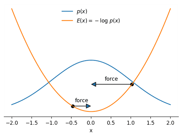
The intuition behind HMC is that we can interpret a random walker as a particle moving under the effect of forces attracting it to higher-probability zones. That is easier to see with an example: in the next image we show both a probability density p(x) and its corresponding negative log-density −logp(x), which we will call the potential energy E(x):
As you can see, the potential energy E(x) looks like a mountainous landscape that attracts the particle (shown at two different positions) to its bottom—the steeper the landscape, the stronger will be the force pulling it towards the bottom. What’s more, the bottom of this landscape coincides with the region with the largest probability of p(x)! That means that if we are able to predict where the particle will move to given its position and velocity, we can use the result of that prediction as a proposal state for a fancy version of Metropolis-Hastings.
This kind of prediction problem is very common and well-studied in physics—think of simulating the movement of planets around the sun, which is determined by gravitational forces. We can thus borrow the well-known theory and methods from classical (“Hamiltonian”) mechanics to implement our method!
While HMC is quite easy to implement, the theory behind it is actually far from trivial. We will skip a lot of detail, but provide additional information on physics and numerics in detailed footnotes.
The HMC algorithm
In physics, the force acting on a particle can be calculated as the derivative (or gradient) of a potential energy E(x). As said above, the negative log-density will play the role of that potential energy for us:
Our particle does not only have a potential energy, but also a kinetic energy, which is the energy stored in its movement. The kinetic energy depends on the particle’s momentum—the product of its mass and velocity. Since in HMC, the mass is often set to one, we will denote the momentum with the letter v (for velocity), meaning that the kinetic energy is defined as1
Just as the position x, the momentum v is generally a vector, whose length is denoted by ∣v∣. With these ingredients in place, we can then define the total energy of the particle as
In classical physics, this quantity completely determines the movement of a particle.
HMC introduces the momentum of the particle as an auxiliary variable and samples the joint distribution of the particle’s position and momentum. Under some assumptions2, this joint distribution is given by
We can sample from p(x,v) efficiently by means of an involved Metropolis-Hastings method: starting from a current state x, we draw a random initial momentum v3 from a normal distribution and simulate the movement of the particle for some time to obtain a proposal state x∗.
When the simulation stops, the fictive particle has some position x∗ and some momentum v∗, which serve as our proposal states. If we had a perfectly accurate simulation, the total energy H(x,v) would remain the same and the final position would be a perfectly fine sample from the joint distribution. Unfortunately, all numerical simulation is only approximative, and we have to account for errors. As we have done before in the original Metropolis-Hastings algorithm, we can correct for the bias with a Metropolis criterion.4 In our case, the acceptance probability is given by
We are not interested in the momentum v∗: if the move is accepted, we only store the position x∗ as the next state of the Markov chain.
Implementation
In terms of implementation, the only part of HMC that is not immediately obvious is the simulation of the particle’s movement. The simulation of the movement of the particle works by discretizing time into steps of a certain size. Position and momentum of a particle are then updated in an alternating fashion. In HMC, this is usually done as follows5:
def leapfrog(x, v, gradient, timestep, trajectory_length):
    v -= 0.5 * timestep * gradient(x)
    for _ in range(trajectory_length - 1):
        x += timestep * v
        v -= timestep * gradient(x)
    x += timestep * v
    v -= 0.5 * timestep * gradient(x)

    return x, v
Now we already have all we need to proceed to the implementation of HMC! Here it is:
def sample_HMC(x_old, log_prob, log_prob_gradient, timestep, trajectory_length):
    # switch to physics mode!
    def E(x): return -log_prob(x)
    def gradient(x): return -log_prob_gradient(x)
    def K(v): return 0.5 * np.sum(v ** 2)
    def H(x, v): return K(v) + E(x)

    # Metropolis acceptance probability, implemented in "logarithmic space"
    # for numerical stability:
    def log_p_acc(x_new, v_new, x_old, v_old):
        return min(0, -(H(x_new, v_new) - H(x_old, v_old)))

    # give a random kick to particle by drawing its momentum from p(v)
    v_old = np.random.normal(size=x_old.shape)

    # approximately calculate position x_new and momentum v_new after
    # time trajectory_length  * timestep
    x_new, v_new = leapfrog(x_old.copy(), v_old.copy(), gradient,
                            timestep, trajectory_length)

    # accept / reject based on Metropolis criterion
    accept = np.log(np.random.random()) < log_p_acc(x_new, v_new, x_old, v_old)

    # we consider only the position x (meaning, we marginalize out v)
    if accept:
        return accept, x_new
    else:
        return accept, x_old
And, analogously to the other MCMC algorithms we discussed before, here’s a function to build up a Markov chain using HMC transitions:
def build_HMC_chain(init, timestep, trajectory_length, n_total, log_prob, gradient):
    n_accepted = 0
    chain = [init]

    for _ in range(n_total):
        accept, state = sample_HMC(chain[-1].copy(), log_prob, gradient,
                                   timestep, trajectory_length)
        chain.append(state)
        n_accepted += accept

    acceptance_rate = n_accepted / float(n_total)

    return chain, acceptance_rate
As an example, let’s consider a two-dimensional Gaussian distribution. Here is its log-probability, neglecting the normalization constant:
def log_prob(x): return -0.5 * np.sum(x ** 2)Now we need to calculate the gradient of the log-probability. Its i-th component is given by ∂xi∂E(x), where xi is the i-th component of the variable vector x. Doing the math, you’ll end up with:
def log_prob_gradient(x): return -xNow we’re ready to test the HMC sampler:
chain, acceptance_rate = build_HMC_chain(np.array([5.0, 1.0]), 1.5, 10, 10000,
                                         log_prob, log_prob_gradient)
print("Acceptance rate: {:.3f}".format(acceptance_rate))
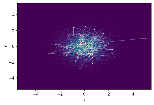
Acceptance rate: 0.622To display the result, we plot a two-dimensional histogram of the sampled states and the first 200 states of the chain:
We see that the HMC states are indeed quite far away from each other—the Markov chain jumps relatively large distances.
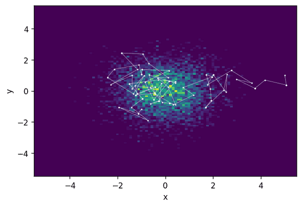
How does Metropolis-Hastings do on the same distribution? Let’s have a look and run a Metropolis-Hastings sampler with the same initial state and a stepsize chosen such that a similar acceptance rate is achieved.
chain, acceptance_rate = build_MH_chain(np.array([5.0, 1.0]), 2.6, 10000, log_prob)
print("Acceptance rate: {:.3f}".format(acceptance_rate))
Acceptance rate: 0.623What you see is that Metropolis-Hastings takes a much longer time to actually find the relevant region of high probability and then explore it. This means that, with a similar acceptance rate, HMC produces much less correlated samples and thus will need fewer steps to achieve the same sampling quality.
While this advantage is even more pronounced in higher dimensions, it doesn’t come for free: numerically approximating the equations of motions of our fictive particle takes up quite some computing power, especially if evaluating the log-probability gradient is expensive.
Choosing the parameters
Two parameters effectively determine the distance of the proposal state to the current state: the integration time step and the number of steps to perform.
Given a constant number of steps, the larger the integration time step, the further away from the current state the proposal will be.
But at the same time, larger time steps implies less accurate results, which means lower acceptance probabilities.
The number of steps has a different impact:
given a fixed step size, the more steps performed, the less correlated the proposal will be to the current state.
There is a risk of the trajectory doubling back and wasting precious computation time, but
NUTS, a neat variant of HMC which optimizes the number of integration steps, addresses exactly this problem.
For a basic implementation of HMC, one can use a fixed number of integration steps and automatically adapt the timestep, targeting a reasonable acceptance rate (e.g. 50%) during a burn-in period.
The adapted timestep can then be used for the final sampling.
Drawbacks
Unfortunately, there’s no such thing as a free lunch. While the big advantage of HMC, namely, less correlated samples with high acceptance rates, are even more pronounced in real-world applications than in our toy example, there are also some disadvantages.
First of all, you can only easily use HMC when you have continuous variables since the gradient of the log-probability for non-continuous variables is not defined. You might still be able to use HMC if you have a mix of discrete and continuous variables by embedding HMC in a Gibbs sampler. Another issue is that the gradient can be very tedious to calculate and its implementation error-prone. Luckily, popular probabilistic programming packages (see below) which implement HMC as their main sampling workhorse, take advantage of automatic differentiation, which relieves the user from worrying about gradients.
Finally, as we just discussed, there are quite a few free parameters, the suboptimal tuning of which can severely decrease performance. However, since HMC is a very popular algorithm, many implementations come with all sorts of useful heuristics to choose parameters, which makes HMC easy to profit from in spite of these drawbacks.
Conclusion
I hope that at this point, you have a general understanding of the idea behind HMC and both its advantages and disadvantages.
HMC is still subject to active research and if you like what you just read (and have the required math / stats / physics knowledge), there are many more interesting things to learn6.
To test your understanding of HMC, here’s a little brain teaser, which also invites you to play around with the code:
what would happen if you made a mistake in the gradient calculation or implementation?
The answer is: you still get a perfectly valid MCMC algorithm, but acceptance rate will decrease.
But why?
I would also like to point out that there are several great, accessible HMC resources out there. For example, a classic introduction is MCMC using Hamiltonian dynamics and these amazing visualizations explain HMC and the influence of the parameters better than any words.
Whether you now decide to take a deep dive into HMC or you’re just content to have finally learned what kind of magic is working under the hood of probabilistic programming packages such as PyMC3, Stan, and Edward—stay tuned to not miss the last blog post in this series, which will be about Replica Exchange, a cool strategy to fight issues arising from multimodality!
- The most general form of the kinetic energy of a physical object is K(v)=2m∣v∣2 with m being the mass of the object. It turns out that HMC even permits a different “mass” (measure of inertia) for each dimension, which can even be position-dependent. This can be exploited to tune the algorithm.↩
- These assumptions are defined by the canonical ensemble. In statistical mechanics, this defines a large, constant number of particles confined in a constant volume. The whole system is kept at a constant temperature.↩
- The temperature of a system is closely related to the average kinetic energy of its constituent particles. Drawing a new momentum for every HMC step can be seen as a kind of thermostat, keeping the average kinetic energy and thus the temperature constant. It should be noted that there are also HMC variants with only partial momentum refreshment, meaning that the previous momentum is retained, but with some additional randomness on top.↩
- HMC combines two very different techniques, both very popular in computational physics: Metropolis-Hastings, which, in a sense, circumvents a real simulation of the physical system, and molecular dynamics, which explicitly solves equations of motion and thus simulates the system. Because of this, HMC is also known as (and was originally named) Hybrid Monte Carlo.↩
- The movement of a classical particle follows a set of differential equations known as Hamilton’s equations of motion. In the context of HMC, numerical methods to solve them have to maintain crucial properties of Hamiltonian mechanics: reversibility assures that a trajectory can be run “backwards” by flipping the direction of the final momentum and is important for detailed balance. Volume conservation essentially keeps the acceptance criterion simple. In addition, symplecticity is highly advantageous: it implies volume conservation, but also guarantees that the energy error stays small and thus leads to high acceptance rates. We use leapfrog integration, which checks all these boxes and is the standard method used in HMC.↩
- How about using differential geometry to continuously optimize the mass or viewing HMC in terms of operators acting on a discrete state space ladder?↩
Behind the scenes
Simeon is a theoretical physicist who has undergone several transformations. A journey through Markov chain Monte Carlo methods, computational structural biology, a wet lab and renowned research institutions in Germany, Paris and New York finally led him back to Paris and to Tweag, where he is currently leading projects for a major pharma company. During pre-meeting smalltalk, ask him about rock climbing, Argentinian tango or playing the piano!
If you enjoyed this article, you might be interested in joining the Tweag team.


