Hamiltonian Monte Carlo (HMC) is a MCMC sampling algorithm which proposes new states based on the simulation of Hamilton’s equations of motion. One of the main ingredients of this algorithm is its integration scheme — how the equations are discretized and its solutions found. The standard choice for this is the classical leapfrog. In this blog post we present our empirical investigation of $U_7$ — an algorithm that is computationally more expensive, but also more accurate. This trade-off is not a simple one (after all, more precision implies less tries), but our explorations show that this is a promising algorithm, which can outperform leapfrog in some cases.

We don’t suppose previous knowledge of integration methods, but in case you are new to HMC or MCMC methods, a good starting point is our blog post series on the subject.

Introduction

Broadly speaking, the idea of HMC is that, given a previous state $x$ of our Markov chain, we draw a random momentum $v$ from a normal distribution and simulate the behaviour of a fictive particle with starting point $(x,v)$. This deterministic behaviour is simulated for some fixed time $t$. The final state $(x^\star, v^\star)$ of the particle after the time $t$ will then serve as the new proposal state of a Metropolis-Hastings algorithm.

The motion of the fictive particle is governed by the Hamiltonian $H(x,v) = K(v) + E(x)$, the sum of the kinetic ($K$) and potential ($E$) energies. The coordinates $(x, v)$ then solve Hamilton’s equations of motions:

By introducing $z=(x,v)$ and defining an operator $D_{H}$, the equations of motion can be written compactly as

The operator $D_{H}$ is a differential operator that uses first derivatives. It describes the change of any observable quantity with respect to the time evolution of a Hamiltonian system. The equations of motion are then formally solved by

Here, $D_K$ and $D_E$ respectively describe the change of $z$ that is due to the kinetic and the potential energy. The full operator $\exp ( t D_H )$ then describes the time evolution of the system — it maps $z(0)$ to $z(t)$. The solution of this equation depends crucially on the potential energy, which in the context of HMC relates to the probability distribution of interest via $E(x) = -\log p(x)$. The density function $p(x)$ is, in general, non-trivial and the Hamiltonian equations of motion can therefore not be solved analytically.

A general recipe for symplectic integration: splitting methods

We thus have to resort to numerical integration to get at least an approximate solution. As discussed in a footnote of Tweag’s HMC blog post, we can’t just use any integration scheme in HMC, but we should make sure it obeys symplecticity. This is a crucial property of Hamilton’s equations of motion and means that they preserve the volume in $(x, v)$ space, ensuring that probabilities are propagated correctly. A very general idea way of deriving symplectic integrators of arbitrary order are splitting methods, as follows.

In 1995, Suzuki proposed a way to approximate expressions such as the formal solution of Hamilton’s equations, yielding in our case

where $\Sigma_{i=1}^k c_i = \Sigma_{i=1}^k d_i =1$. You can think of this formula as a generalization of the identity $e^{m+n} = e ^m \cdot e^n$ to operators. The error term is a result of the fact that operators generally do not commute.

The factors $\exp (c_i t D_K)$ correspond to an update of the position $x$, while the $\exp (d_i t D_E)$ correspond to an update of the momentum $v$.¹

Now, that we know how to come up with an approximation of the solution of the equations of motion, let’s give a first example of an approximative algorithm.

The Leapfrog

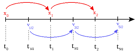
The Leapfrog algorithm is the standard integrator used in HMC. The intuition behind it is that we alternate updating the position coordinate $x$ and the momentum variable $v$, but half a time step apart:

(source: Steve McMillan, Drexel University)

This behaviour has given the Leapfrog algorithm its name. More precisely, the updates look like the following,

As you might have noticed, you need to perform half a step for the momentum in the beginning and in the end. So, in terms of Suzuki, the Leapfrog looks like this

where

The coefficients are $c_1 = 0,\, c_2 = 1,\, d_1=d_2 = \frac{1}{2}.$

If we further divide our time $t$ into $t = \text{time\ step} \cdot \text{trajectory\ length}$ and apply the Suzuki approximation $U_3$ $\text{trajectory\ length}$-many times, we can implement this in Python as follows:

def integrate(x, v):

    v += 1 / 2 * time_step * -gradient_pot_energy(x)

    for i in range(trajectory_length - 1):
        x += time_step * v
        v += time_step * gradient_pot_energy(x)

    x += time_step * v
    v += 1 / 2 * time_step * gradient_pot_energy(x)

    return x, v

An important concept when talking about the accuracy of integration schemes is that of the order of an integrator: if $(x^\star,v^\star)$ is the exact solution after time $t$ and $(x_{t},v_{t})$ an approximation, then we say that the approximation is of nth-order and write $\mathcal{O}(t^n)$, if $\Vert(x^\star,v^\star)-(x_{t},v_{t}) \Vert\leq C \cdot t^n$ and $C$ is independent of $t$.

One can verify that the $U_3$ is exact to first-order in $\Delta t$.² Furthermore, because of symmetry, the $U_3$ needs to be of even-order.³ Thus the $U_3$ cannot be only a first-order approximation — it needs to be correct up to $\Delta t ^2$. In this sense, the $U_3$ is a second-order approximation and the Leapfrog is too.

Now, you might wonder: why look further since we have found a method yielding a reasonably exact approximation? After all, we can always diminish the error by shortening the time step and increasing the trajectory length!

Well, one answer is that there might be a more efficient way to approximate the equations of motions!

The $U_7$

A seven-factor approximation, $U_7$, which can be molded into a five-factor form and which has fourth-order accuracy (that is, it is more precise than leapfrog), was first considered by Chin (1997). Its novelty lies in the usage of the second-order derivative of the potential energy. This comes along with a few more updates of $x$ and $v$ per step. A rediscovery by Chau et al. builds on Suzuki’s method discussed above, but is focused on quantum mechanical applications. We now sketch Chin’s more accessible way of deriving the $U_7$.

When we want to apply $e ^A \cdot e^B \cdot e^C= e^{A+B+C}$ to operators, we remember that we must take into account that they do not commute — therefore, this identity thus does not hold in the general case. However, we can use a series expansion, which, like a Taylor expansion, in our case involves higher order derivatives. Then, cutting off the expansion leaves us with an additional error, which is of order $\mathcal{O}(\Delta t^5)$. Consequently, the $U_7$ remains exact up to the fourth order.

Whichever way the $U_7$ is derived, the newly formed term involves the second order derivative and the final $U_7$ factorization is given by

$U_7 = \exp \left(\frac {1}{6}\Delta t D_E\right)\exp \left(\frac {1}{2}\Delta t D_K\right)\exp \left(\frac {2}{3}\Delta t D_{\tilde{V}}\right)\exp \left( \frac {1}{2}\Delta t D_K\right)\exp \left(\frac {1}{6}\Delta t D_E\right),$

whereas $D_{\tilde V}$ is a differential operator reflecting the influence of a modified potential energy $V + \frac{1}{48}[\Delta t\nabla V ]^2$ and is thus effectively a second-order derivative.

A Python implementation of the algorithm described above would look like this:

def integrate(x, v):

    v += 1 / 6 * time_step * gradient_pot_energy(x)

    for i in range(trajectory_length - 1):
        x += 1 / 2 * v * time_step
        v += (2 / 3 * time_step * (gradient_pot_energy(x)
            + time_step ** 2 / 24
            * np.matmul(hessian_log_prog(x),gradient_pot_energy(x))))
        x += 1 / 2 * v * time_step
        v += 1 / 3 * time_step * gradient_pot_energy(x)

    x += 1 / 2 * v * time_step
    v += (2 / 3 * time_step * (gradient_pot_energy(x)
        + time_step ** 2 / 24
        * np.matmul(hessian_log_prog(x),gradient_pot_energy(x))))
    x += 1 / 2 * v * time_step
    v += 1 / 6 * time_step * gradient_pot_energy(x)

    return x, v

Bear in mind that the higher accuracy achieved with $U_7$ comes with a non-negligible additional computational cost, namely evaluating the gradient two times instead of one time and additionally evaluating the matrix of second derivatives.

Benchmarking leapfrog and $U_7$-based HMC

In this paper, Jun Hao Hue et al. benchmark the performance of the leapfrog and $U_7$ against various classical and quantum systems, but are not concerned with their use in HMC.

To compare the performance of the leapfrog and U7 integration schemes in the context of HMC, we plug above implementations into HMC and sample from two different probability distributions.

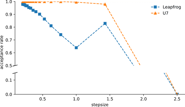
The first example is a 100-dimensional standard normal distribution. Because of the high symmetry of this distribution, we must be careful to not compare apples and oranges: if we integrate for different total times, the trajectory might double back and we would waste computational effort — avoiding this is the goal of a widely popular HMC variant called NUTS. We thus fix the total integration time (given by number of integration steps x time step) to ten-time units and run HMC for different combinations of time step and number of integration steps. If we can use a higher time step, we have to perform less integration steps, which means less costly gradient and Hessian evaluations.

We find indeed that the acceptance rate for $U_7$ stays almost constant at almost one for a wide range of time steps, while the HMC implementation based on the leapfrog integration scheme shows rapidly diminishing acceptance rates. We currently cannot explain the local maximum in the Leapfrog acceptance rate around a stepsize of $1.5$, but we suspect it has to do with high symmetry of the normal distribution — perhaps the Leapfrog is, for that stepsize / trajectory length combination, performing an additional U-turn that makes it double back towards more likely states. In any case, this confirms that we have implemented the U7 integrator correctly and makes us even more excited to test it on a “real” system!

As a more practical application, we consider a simple, coarse-grained polymer model which could represent a biomolecule, like a protein or DNA. In Bayesian biomolecular structure determination, one seeks to infer the coordinates of atoms or coarse-grained modelling units (monomers) of such a polymer model from data obtained from biophysical experiments. This results in an intractable posterior distribution and MCMC methods such as HMC are used to sample from it.

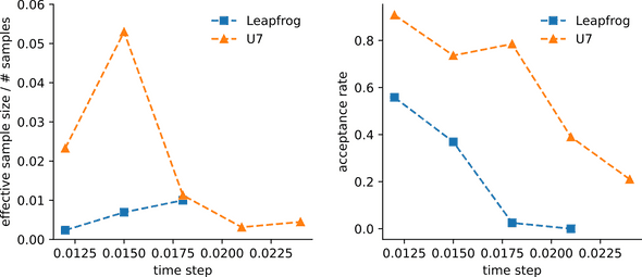
In our case, we consider a polymer of $N=30$ spherical particles with fictive springs between neighbouring particles. We also include a term that makes sure particles do not overlap much. Furthermore, we assume that we have measured pairwise distances for two particle pairs and that these measurements are drawn from a log-normal distribution. See this article for details on a very similar model. This setup results in a posterior distribution over $N \times 3=90$ parameters, from which we sample using HMC with either the leapfrog or the $U_7$ integrator. Drawing 10000 samples with a trajectory length of ten steps and varying time steps, we find the following results for the effective sample size (ESS) of the log-posterior probability and the acceptance rate:

We find that, just as for the 100-dimensional normal distribution, the $U_7$ HMC shows significantly increased acceptance rates as compared to the leapfrog HMC. The calculation of the ESS shows that for the two smallest time steps tested, the estimated number of independent samples is much higher for the $U_7$-based HMC than for the standard implementation. It is important to note that in our experiments, if the acceptance rate gets very low, the ESS is likely vastly overestimated. We omit these erroneous data points and can suspect that also for the third time step, the ESS obtained with standard HMC is probably smaller than shown.

Analysis of benchmark results

What does this mean with respect to absolute performance? Remember that while the $U_7$ yields better acceptance rates and higher ESS, it also requires more computing time: The computationally most expensive part of both integrators is evaluating the first and second derivatives of the log-probability. This requires, in both cases, the evaluation of all pairwise Euclidean distances between monomers. In both cases, the distance evaluations are dominating the computational cost. We assume thus that the computational cost for evaluating the gradient and the second derivative is identical and equal to the cost of evaluating all pairwise distances. Note that we neglect all additional, implementation-specific overhead.

Under these coarse assumptions, we can thus estimate the computational effort for a $U_7$ iteration to be approximately twice the effort of a leapfrog iteration. Given that, based on the ESS estimation, we can achieve up to approximately seven times the number of independent samples with $U_7$, we conclude that the $U_7$ integrator indeed is a very promising way to boost HMC performance.

Conclusion

I hope that you have gained a deeper understanding of the numeric behind Hamiltonian mechanics and that this blog post stimulated you to think more about alternative integration schemes for HMC. Symplectic integration is still an active field of research and especially its applications outside physics are just being explored - we surely can expect more cool results on different integration schemes in the future!

Put in a nutshell, we have seen that HMC does not necessarily rely on the leapfrog integrator and may even be better off with higher-order integration schemes such as $U_7$.